5 Best Excel Functions You Need in 2022

Microsoft Excel is everywhere in the world of work.
Given this is makes sense to learn Excel properly and make yourself more productive.
According to a recent survey by Excel Skills survey by Acuity Training just 33% of people rank themselves as advanced Excel users or better despite the time they spend using Excel.
To help people improve in this article Acuity Training has highlighted 5 features of Excel that everyone should learn in 2022.
NOTE: Dynamic array functionality was introduced in Excel 365 and Excel 2019 versions. Older versions support dynamic arrays but it is not native.
1. XLOOKUP
Lookup functions are extremely useful allowing you to find data using data in other columns and rows as the criteria.
In the older versions of Excel, it was supported by VLOOKUP, HLOOKUP, and LOOKUP functions.
In Excel 365, Microsoft has introduced the XLOOKUP function in place of these functions as it is much more flexible and dynamic.
XLOOKUP has the following arguments
=XLOOKUP(lookup_value, lookup_array, return_array, [if_not_found], [match_mode], [search_mode])
Lookup_value – Refer to the value that you want to search from the data
Lookup_array – Refers to the range to look up the value from
Return_array – Refers to the range containing the output if the value is found
[If_not_found] – Optional; Value to return if the value is not found
[match_mode] – Optional; 0 = exact match (by default), -1 = exact or next smallest match, 1 = exact or next larger match, 2 = wildcard entries
[search_mode] – Optional; 1 = search from first value in the array (default), -1 search from the last value
The example below shows a basic XLOOKUP in action.
Here XLOOKUP is used to look up the ‘Salary’ of the employee against the ‘Employee ID’.
In cell G4, the XLOOKUP formula is used by:
- Assigning cell G3 as lookup_value,
- B3:B7 assigned as lookup_array and
- D3:D7 assigned as return_array

2. Co-authoring
When working collectively on a project, we often come across a situation where two or more persons need to work on the same workbook.
Previously, this wasn’t possible, which led to no end of issues with version control on large Excel sheets.
Now Excel has introduced the Co-authoring feature from the Excel 365 and Excel 2019 versions.
It allows teams to all work on the same workbook at the same time.
Sharing a workbook takes just a couple of simple steps.
Before sharing the workbook with other members, first, you need to upload the workbook on OneDrive or Microsoft SharePoint.
Once the workbook is uploaded to the cloud, you can easily share it with your peers by clicking on the SHARE button located at the top right corner of your Excel window.
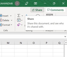
After clicking the share button, you enter the email addresses of the people you’d like to share the workbook with.

3. Dynamic Arrays
Dynamic arrays are one of Excel most recent updates.
They make working with formulas that return multiple inputs very simple to work with.
You don’t need to copy the formula to the last row anymore.
With dynamic arrays, you can get multiple outputs with a single formula.
Let’s look at using dynamic arrays with a simple LEFT function.
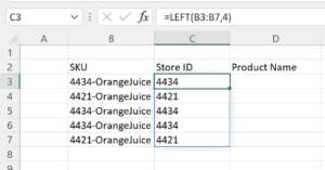
The LEFT function helps extract the required set of characters from the text.
Here we have extracted the Store ID from the SKU column. We have only input the formula into Cell C3 and Excel has completed the result in C4 to C7.
Cell B3:B7 is the range that we want to extract the Store ID to.
By mentioning the range in the function, Excel automatically identifies the range we need and has return multiple results.
Dynamic arrays are a huge topic so if you would like to learn more see Microsoft’s article on dynamic arrays.
4. MAXIFS and MINIFS
MAXIFS and MINIFS come in handy when you need to summarise data quickly.
Both functions can return values based on multiple criteria, and the criteria can include dates, text, numbers, and other data types.
MAXIFS is used to return the maximum value from the range based on one or more criteria.
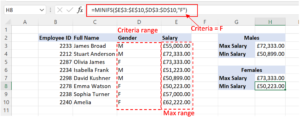
MINIFS is used to return the minimum value from the range based on one or more criteria.
The arguments for both functions are similar
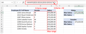
=MAXIFS(max_range, criteria_range1, criteria1,…)
Max_range – Refers to the range of value you want the value to be returned
Criteria_range1 – Refers to the range for the first condition
Criteria1 – Refers to the condition to be used to return the value
The example below shows MAXIFS in action.
Similarly, for MINIFS,
5. Shortcut Keys
Excel has a huge number of shortcut keys.
You don’t need to learn all of them but learning the top 10 or 20 will make you far faster.
Some of the most important and commonly used shortcut keys are:
- CTRL + DOWN: Navigates to the last cell of the data
- CTRL + UP: Navigates to the topmost cell of the data
- CTRL + RIGHT: Navigates to the rightmost cell of the data
- CTRL + LEFT: Navigates to the leftmost cell of the data
- CTRL + Z: Undo last action
- CTRL + Y: Redo the previous action
- CTRL + O: To open the workbook
- CTRL + S: To save the workbook
- CTRL + N: Creates a new workbook
- CTRL + 1: Opens the Format Cells dialog box
- ALT + Enter: For line break within the cell
- CTRL + C: Copy the selected cell(s)
- CTRL + V: Paste the copied/cut cell
- CTRL + ALT + V: Open the paste special dialog box
- CTRL + T: Insert table
- F4: Repeats the last action
This article contains a full list of Excel shortcuts.
Final Thoughts
Learning the 5 skills above will speed up your day-to-day work significantly.
If you practice them when you have 5 minutes spare you’ll be surprised how much time they save you.
Write For Us
Gain multichannel inventory visibility and control with eChannelHub
Learn more about eChannelHub with a free demo, tailored for your unique retail business.
Request A DemoRequest a Demo
Gain multichannel inventory visibility and control with eChannelHub
Learn more about eChannelHub with a free demo, tailored for your unique online business


